
Aims -
- Introduction to spark/XGBoost/tensorflow - large scale data analysis frameworks
- Use stats and ML to analyze and identify statistically significant patterns and visually summarize them
Topics -
- Memory Hierarchy
- Spark Basics
- Dataframes & SQL
- PCA and weather analysis
- K-means and intrinsic dimensions
- Decision trees, boosting, random forests
- Neural networks & tensorflow
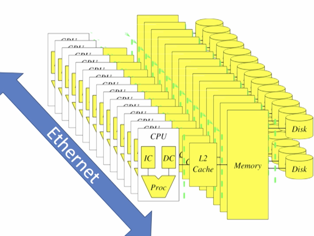
Memory Hierarchy Latency of read-write > latency of computation Main memory faster than disk
Temporal locality and spatial locality e.g. count words by sorting Spatial -> memory is stored in blocks not single bytes. Blocks are moved from disk to memory thus the surrounding nearby data is already in memory. Spatial locality makes code faster (x300)
Access locality - cache efficiency. (Try to reuse the same memory elements/blocks repeatedly)
- Temporal locality - accessing the same elements again and again in quick succession, e.g. theta vector of a neural network
- Spatial locality - access elements close to each other e.g. indexed array will store elements in same pages/blocks and as soon as the page is copied into the cache, consecutive pairs of array elements will already be cached
Row major vs column major layout - if row major then row-wise traversal is faster than column by column traversal. (e.g. in numpy)
Measuring latency, studying long-tail distributions Memory latency: time between CPU issuing a command and when the command completes. Time is short if element is already in L1 cache, long if element is in disk/SSD.
Using CDF and loglog plotting, we can see that probability of extreme values (long-tail) is higher than what mean/normal distribution etc would indicate. (Long tail distribution - a distribution far from normal distribution graph line)
Sequential access is much much faster than random access. Writing memory sequentially makes it faster than simple unitary method multiplication logic. Bandwidth vs latency e.g. it takes 8.9s to write 10GB to SSD but that doesn’t imply it takes 8.9 * 10^-10s to write a single byte. Many write ops occur in parallel. Byte rate for writing memory - 100MB/sec, SSD - 1GB/sec
When reading/writing large blocks, throughput is important, not latency (economies of scale)
Data analytics: moving data around/data access is the bottleneck, NOT computation clock speed
Caching is used to transfer data b/w different levels of memory hierarchy. (Registers/L1/L2/main memory/disk). To process big data, we need multiple computers.
Cluster - collection of many computers connected by ethernet.
Abstraction needed to transfer data between computers and hidden from programmers. In Spark, this is the Resilient Distribution Dataset.
How is data distributed across a cluster? Each file is broken into chunks, (kept track of by chunk master) and each chunk is copied and distributed randomly across machines. GFS/HDFS: Break files into chunks, make copies, and distribute randomly among commodity computers in a cluster
-Commodity hardware is used.
-locality: each data is stored close to a CPU so can do some computation immediately without needing to move data
-redundancy: can recover from hardware failures
-abstraction: designed to look like a regular filesystem, chunk mechanism is hidden away
MapReduce: Computation abstraction that works well with HDFS. No need to take care of chunks/copies etc
Spark Basics
Square each number in a list -
[x*x for x in L]
OR
map(lambda x:x*x, L) [order of elements is not specified]
Sum each number in a list -
s = 0; for x in L: s += x
OR
reduce(lambda (x,y): x+y, L) [order of computation is not specified]
Compute sum of squares of each number in a list -
S = 0; for x in L: s += x * x
OR
reduce(lambda (x,y): x+y, map(lambda i:i*i, L))
Computation order specified vs not specified Immediate execution vs execution plan Map/reduce ops should not depend on : order of items in list (commutativity) / order of operations (associativity) Order independence - result of map/reduce does not depend on order of input. Allows parallel computation, allows compiler to optimize execution plan
Spark is different from Hadoop: stores distributed memory instead of distributed files Core programming language for Spark: Scala
Spark Architecture:
Spark Context - connects our software to controller node software that controls the whole cluster. We can control other nodes using the sc object. sc=SparkContext()
Resilient Distributed Dataset (RDD): a list whose elements are distributed over multiple nodes. We may perform parallel operations on this list using special commands, which are based on MapReduce RDDs are created from a list on the master node or a distributed HDFS file. ‘Collect’ command is used to translate into local list.
RDD = sc.parallelize([0,1,2])
RDD.map(lambda x:x*x).reduce(lambda x,y:x+y)
^we don’t have direct access to elements of the RDD
A = RDD.map(lambda x:x*x) //0,1,2
A.collect() //0,1,4
We may take first few elements of a RDD
B = sc.parallelize(range(10000))
print B.first
print B.take(5)
print B.sample(False,5/10000).collect() // samples 5 random elements
Master->Slave architecture
Cluster Master manages the computation resources. Each worker manages a single core. Driver(main() code) runs on the master. (Spatial organization)
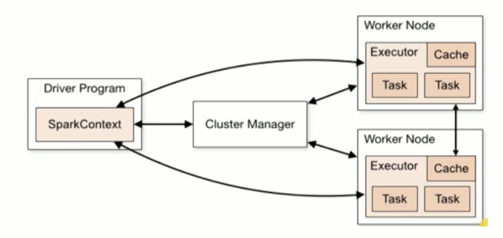
RDDs are partitioned across the workers. Workers manage these partitions and the executors. SparkContext is an encapsulation of the cluster for the driver node. Worker nodes communicate with Cluster Manager.
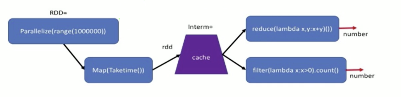
Materialization - intermediate RDDs don’t need to be stored in memory (materialized). RDDs by default are not materialized. They are stored if cached - forced calculation of intermediate results.
Stage - set of operations that can be done before materialization is necessary i.e. compute one stage, store the result, compute next stage etc (temporal organization)
Execution concepts -
* RDDs are partitioned across workers
* RDD graph defines the lineage of RDDs
* SparkContext divides RDD graph into Stages which define the execution plan
* a Task is for one stage, for one partition. Executor is the process that performs tasks. Thus tasks are divided by temporal (stage) and spatial (partition) concepts
Spatial vs Temporal organization : data partitions are stored in different machines vs computation performed in sequence of stages
Plain RDDs: parallelized lists of elements Types of commands:
- Creation : RDD from files/databases
- Transformations: RDD to RDD
- Actions: RDD to data on driver node/files e.g. .collect(), .count(), .reduce(lambda x:x * x) [sum the elements]
Key-value RDDs: RDDs where elements are a list of (key, value) pairs
car_count = sc.parallelize((‘Honda’, 2), (’subaru’, 3), (‘Honda’, 2))
// create RDD
A = sc.parallelize(range(4)).map(lambda x : x*x)
A.collect() // action
B = sc.parallelize([(1,3), (4,5), (-1,3), (4,2)])
B.reduceByKey(lambda x,y: x*y) // each key will now appear only once
 .collect() // [(1,3),(-1,3),(4,10)]
groupByKey: returns a (key,
.countByKey() - returns dictionary with (key, count) pairs for each key
.lookup(3) - returns all values for a key
.collectAsMap() - like collect() but returns a map instead of a list of tuples. Each key is mapped to the list of values associated with it
Example - find longest and alphabetically last word in a list using Reduce
def last_largest(x, y):
    if len(x) > (y): return x
    elif len(y) > (x): return y
    else:
        if x > y: return x
        else: return y

wordRDD.reduce(last_largest)
Programming Assignment 1 - Q. Given an input file with an arbitrary set of co-ordinates, your task is to use pyspark library functions and write a program in python3 to find if three or more points are collinear. For instance, if given these points: {(1,1), (0,1), (2,2), (3,3), (0,5), (3,4), (5,6), (0,-3), (-2,-2)} Result set of collinear points are: {((-2,-2), (1,1), (2,2), (3,3)), ((0,1), (3,4), (5,6)), ((0,-3), (0,1), (0,5))}. Note that the ordering of the points in a set or the order of the sets does not matter.
Solution -
def format_result(x):
    x[1].append(x[0][0])
    return tuple(x[1])

def to_sorted_points(x):
    return tuple(sorted(x))

def to_tuple(x):
    x1 = x.split()
    return (int(x1[0]), int(x1[1]))

def find_slope(x):
    if x[1][0] - x[0][0] == 0:
        return ((x[0], 'inf'), x[1])

    m = (x[1][1] - x[0][1])/(x[1][0] - x[0][0]) # slope = y2 - y1 / x2 - x1
    return ((x[0], m), x[1])

def non_duplicates(x):
    mapping = {}
    for i in range(len(x)):
        if x[i] in mapping:
            return False
        mapping[x[i]] = True
    return True

def get_cartesian(rdd):
    rdd1 = rdd.cartesian(rdd)
    rdd2 = rdd1.filter(non_duplicates)
    return rdd2

def find_collinear(rdd):
    rdd1 = rdd.map(find_slope) # get slope for each pair of points
    rdd2 = rdd1.groupByKey().mapValues(list) # group the values for each key - hash-partition
    rdd3 = rdd2.map(lambda x: format_result(x)).filter(lambda x: len(x) > 2) # format and keep only >2 point lists

    return rdd3

def build_collinear_set(rdd):
    rdd = rdd.map(lambda x: to_tuple(x))
    rdd = get_cartesian(rdd)
    rdd = find_collinear(rdd)
    rdd = rdd.map(to_sorted_points)

    return rdd

# test the above methods
from pyspark import SparkContext, SparkConf
conf = SparkConf().setAppName("Collinear Points").setMaster("local[4]") #Initialize spark context using 4 local cores as workers
sc = SparkContext(conf=conf)

from pyspark.rdd import RDD
test_rdd = sc.parallelize(['4 -2', '2 -1', '-3 4', '6 3', '-9 4', '6 -3', '8 -4', '6 9'])
assert isinstance(build_collinear_set(test_rdd), RDD) == True, "build_collinear_set should return an RDD."
When we start SparkContext, we can specify the number of workers - usually 1 worker per core. More than 1 worker/core doesn’t increase speed much.
Spark Internals
Lazy Evaluation: no need to store intermediate results, scan through data only once. e.g. processing 1 million rows with an op that takes 25us doesn’t take 25s.
No computation is done immediately, only an execution plan is defined using a dependence graph for how RDDs are computed from each other. We can print the dependence graph using rdd.toDebugString(). We may cache (materialize) the results. (.cache()). Thus when RDDs are reused, it’s better to materialize them.
Partitions & Gloming
We can specify no of partitions for a RDD to be distributed into (default - no of workers/cores). Sometimes if the data in diff partitions become unbalanced (e.g. by filtering, some partitions have no data), we have to repartition the RDD.
Glom is used to refer to individual elements. Glom() transforms each partition into a tuple of elements - creates a RDD of tuples, thus can access the elements as lists.
Eg used to count no of elements in each partition - rdd.glom().map(len).collect() prints a list like [20, 43] etc.
Chaining
Sequential vs Pipelined Execution - no intermediate results stored, only 1 pass through input RDD, less memory required
B.sample(False, m/n) - sampling a RDD. Aggregates like avg can be approximated using a sample. Gives different size list each time. (Parameters - with/without replacement, probability of taking an element)
B.filter(lambda x : x%2) - filtering a RDD
B.distinct() - removes duplicate elements. This is a shuffle operation - lot of communication required
.flatMap() - assumed .map() command generates a list and concatenates the items
Set operations - A.union(B)/A.intersection(B)/A.subtract(B)/A.cartesian(B)
Word Count
- Split line by space
- Map word to (word,1)
- Count no of occurrences of each word
text_file = sc.textFile(file path)
type(text_file)
words = text_file.flatMap(lambda line: line.split(“ “)) // one long RDD formed
not_empty = words.filter(lambda x : x != ‘ ‘)
key_values = not_empty.map(lambda x : (x, 1))
counts = key_values.reduceByKey(lambda x, y: x + y)
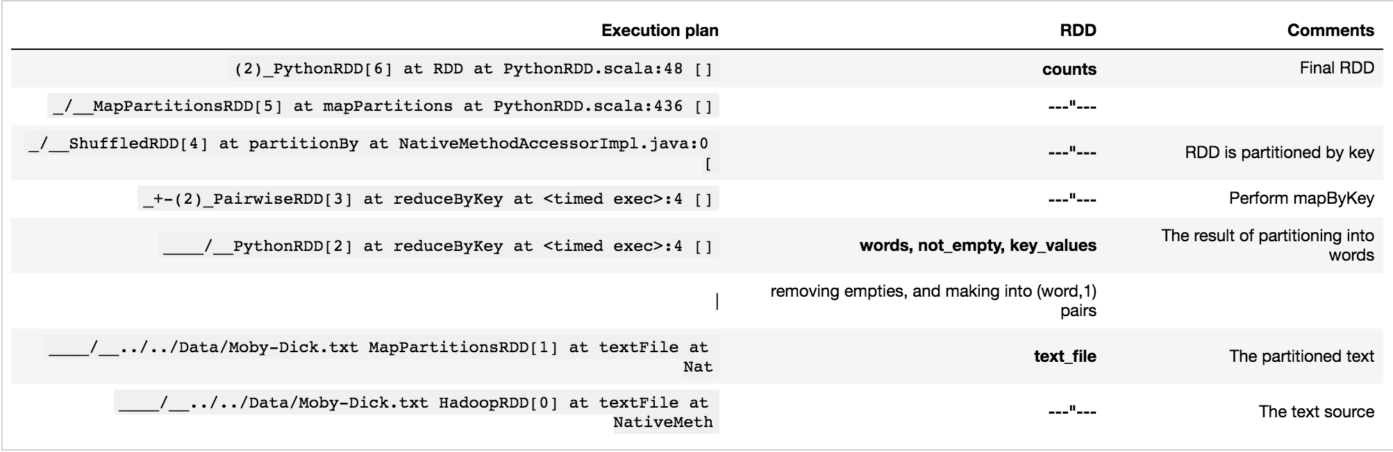
During execution, Spark will materialize (cache) key_values RDD because reduceByKey requires a shuffle, for which the input RDD must be materialized.
After collect/reduce, any code is executed on the head node - Spark parallelism is not utilized after that.
Find 5 Most Frequent Words
- collect and sort on head node
- collect only at the end (faster using Spark efficiency) - collect to the head node only more frequent words
word_pairs = textFile.flatMap(lambda x : x.split(" ")).filter(lambda x : x != " ").map(lambda x: (x, 1))
count = word_pairs.reduceByKey(lambda x, y: x + y)

// Now to sort according to count, we have to have count as key and word as value. So reverse current pair order
reverse_counts = count.map(lambda x: (x[1], x[0]))
sorted_counts = reverse_counts.sortByKey(ascending=False)
result = sorted_counts.take(5) // actually executed the plan - computation starts here
Spark Operations -
- Transformations e.g. map, filter, sample - no/very little communication needed b/w RDDs
- Actions e.g reduce, collect, count, take - more communication, generates result in the head node
- Shuffles e.g. sort, distinct, sortByKey, reduceByKey, join, repartition - a lot of communication required - slowest
.groupByKey - returns a RDD of (key,
e.g. [(1,2), (2,4), (2,6)] -> [ (1, [2]), (2, [4, 6]) ]
.flatMapValues - create a k-v pair for each element of the list generated by the flatMap
e.g. [(1,2), (2,4)] -> [(1,2), (1,3), (2,4), (2,5)]
Join - merges rows with same key between 2 RDDs. e.g. join called on 2 datasets - (key, V) and (key, W) - produces (key, (V, W)) with all pairs of elements for each key.
DataFrames & SQL
Store 2-dimensional data, like rows & columns. Columns can have different types. A dataframe is a RDD of rows plus some high-level schema information. We can construct a data frame from a RDD of rows -
rdd1 = sc.parallelize([Row(name=“John”, age=19), Row(name=“Sid”, age=33), Row(name=“Jlai”, age=28)])
df = sqlContext.createDataFrame(rdd1)
df.printSchema()
Or we can use a regular RDD plus a schema by passing a StructType schema
Rdd2 = sc.parallelize([("John", 19), (“Sid", 23), (“Hzor", 18)])
schema = StructType([StructField("name", StringType(), False), StructField(“age", IntegerType(), False)])
df = sqlContext.createDataFrame(rdd2, schema)
df.printSchema()
Usually load the DataFrame from disk - json/csv/parquet.
Parquet - a popular columnar format to store data frames on disk. We can use Spark SQL to query the file directly and only relevant parts of the file are retrieved (instead of fetching the whole file). Compatible with HDFS/parallel retrieval & column-wise compression is also possible (in case of duplicate column values)
Dataframes can be stored/retrieved from parquet files. We can directly refer to parquet file in a SQL query
df = sqlContext.read.load(parquet_filename)
df.show()
df.select(“name”, “age”)
Imperative vs Declarative Manipulation Imperative - how you want to compute e.g.
df.groupby(‘measurement’).agg({‘year’:’min’, ’city’: ‘count'}).show()
df.agg({‘measure’: ‘approx_count_distinct’}).show() # sampling gives slightly diff results each time
Declarative - describe what you want to compute. Compiler will optimize it. Disadvantage - sometimes low-level primitives are not present e.g. covariance e.g.
#  we need to register a data frame as a table before running SQL on it.
sqlContext.registerDataFrameAsTable(df,'weather’)

query = “SELECT measure, COUNT(measure) as count, MIN(year) FROM weather GROUP BY measure ORDER BY count”
sqlContext.sql(query).show()
We need to register UDFs (User Defined Functions) for custom logic before applying them in a data frame e.g.
def count_nan(V):
    A = unpackArray(V, data_type=np.float16)
    return sum(np.isnan(A))
count_nan_udf = udf(count_nan, IntegerType())

weather_df.withColumn(“nan_no”,count_nan_udf(weather_df.Values))
Before we analyze a large data set, it’s important to know how dense is it. Find out by plotting histograms - reduce the relevant columns using reduceByKey() and use pandas to plot.
Moving & Deserializing Data - takes a big part of the execution time.
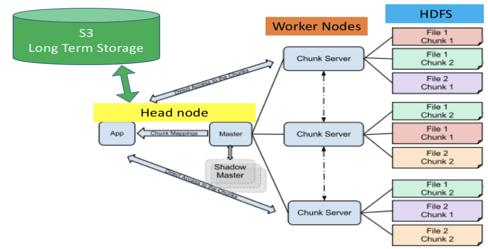
S3 is used for long term storage. We put data from S3 to head node and then from head node to HDFS so workers can process tasks on the data. S3 -> head node (serial to serial movement) head node -> HDFS (serial, uses Hadoop command)
Now the file has been distributed in small chunks across worker nodes. P.S. parallelization is not always faster (generally useful when the data is too large for a single node’s memory)
Overall Flow:
- Define schema and transform RDD to dataframe
- Save data frame as a parquet file
- Copy parquet to head node and S3
- Efficient to keep data in parquet files on S3